2 Manipulator kinematics
This Notebook illustrates how the manipulator will arrive at the desired location as instructed by the speech input.
2.1 Forward and Inverse Kinematics
Kinematics is the science of motion that treats the subject without regard to the forces that cause it.
2.1.1 Forward Kinematics
Forward kinematics addresses the problem of computing the position and orientation of the end effector relative to the user’s workstation given the joint angles of the manipulator.
The forward kinematics were performed in accordance with the Denavit—Hartenberg (D-H) convention. According to the D-H convention, any robot can be described kinematically by giving the values of four quantities, typically known as the D-H parameters, for each link. The link length a and the link twist \alphaquantities, describe the link itself and the remaining two; link offset d and the joint angle \theta describe the link’s connection to a neighboring link.
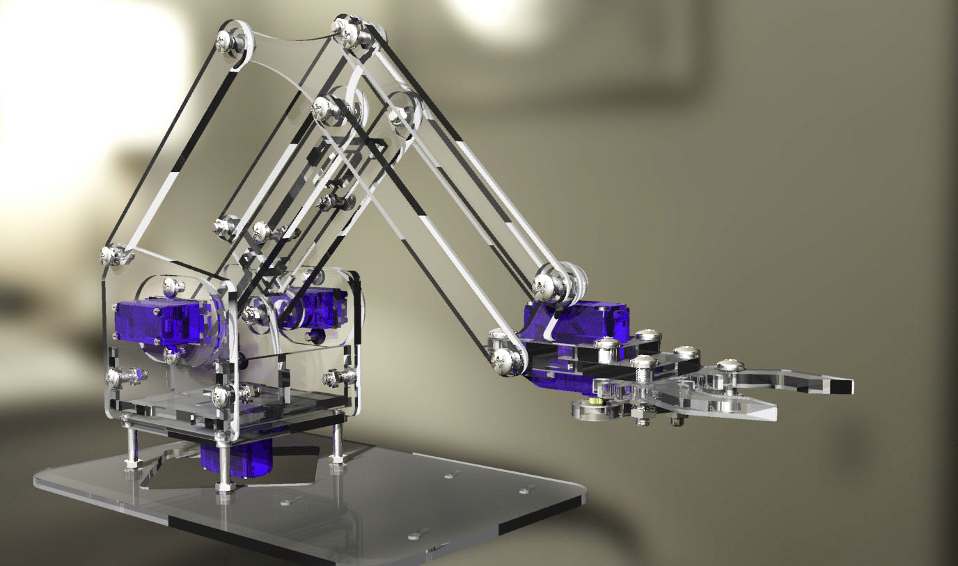
To perform the manipulator kinematics, link frames were attached to the manipulator as shown in Figure 2.1. In summary, link frames are laid out as follows:
- The z-axis is in the direction of the joint axis.
- The x-axis is parallel to the common normal.
- The y-axis follows from the x-axis and z-axis by choosing it to be a right-handed coordinate system.

Once the link frames have been laid, the D-H parameters can be easily defined as:
d: offset along the previous z to the common normal.
\theta: angle about previous z, from old x to new x.
a: length of the common normal.
\alpha: angle about common normal from old z\ axis to new z\ axis.
The D-H parameters for the meArm were evaluated as below:
| Link | \theta | a(mm) | \alpha | d(mm) |
|---|---|---|---|---|
| 1 | \theta_1 | 0 | 90 | 55 |
| 2 | \theta_2 | 80 | 0 | 0 |
| 3 | \theta_3 | 120 | 0 | 0 |
In this convention, each homogeneous transformation A_i is represented as a product of the four basic transformations (Spong, Hutchinson, and Vidyasagar 2005), which evaluates to a 4\times4 matrix that is used to transform a point from frame n to n\ -1.
A_i = Rot_{z, \theta_i}\ Trans_{x, a_i}\ Rot_{x, \alpha_i} \\
= \begin{bmatrix} c_{\theta_i} & -s_{\theta_i} & 0 & 0 \\ s_{\theta_i} & c_{\theta_i} & 0 & 0 \\ 0 & 0 & 1 & 0 \\ 0 & 0 & 0 & 1 \end{bmatrix} \begin{bmatrix} 1 & 0 & 0 & 0 \\ 0 & 1 & 0 & 0 \\ 0 & 0 & 1 & d_i \\ 0 & 0 & 0 & 1 \end{bmatrix}\\ \times \begin{bmatrix} 1 & 0 & 0 & a_i \\ 0 & 1 & 0 & 0 \\ 0 & 0 & 1 & 0 \\ 0 & 0 & 0 & 1 \end{bmatrix} \begin{bmatrix} 1 & 0 & 0 & 0 \\ 0 & c_{\alpha_i} & -s_{\alpha_i} & 0 \\ 0 & s_{\alpha_i} & c_{\alpha_i} & 0 \\ 0 & 0 & 0 & 1 \end{bmatrix}
\begin{bmatrix} c_{\theta_i} & -s_{\theta_i}c_{\alpha_i} & s_{\theta_i}c_{\alpha_i} & a_ic_{\theta_i} \\ s_{\theta_i} & c_{\theta_i}c_{\alpha_i} & -c_{\theta_i}s_{\alpha_i} & a_is_{\theta_i} \\ 0 & s_{\alpha_i} & c_{\alpha_i} & d_i \\ 0 & 0 & 0 & 1 \end{bmatrix}
Considering the three links of the meArm, the total homogeneous transformation will be a product of the transformations of the three links given as:
A_T = A_1 \times A_2 \times A_3 \tag{2.1}
The final total homogeneous transformation was derived to be:
A_t =\ \begin{bmatrix} cos(\theta_2 + \theta_3)cos(\theta_1) & -sin(\theta_2 + \theta_3)cos(\theta_1) & sin(\theta_1) & 4\sigma_1cos(\theta_1) \\cos(\theta_2 + \theta_3)sin(\theta_1) & -sin(\theta_2 + \theta_3)sin(\theta_1) & -cos(\theta_1) & 4\sigma_1sin(\theta_1) \\ sin(\theta_2 + \theta_3) & cos(\theta_2 + \theta_3) & 0 & 12sin(\theta_2 + \theta_3) + 8sin(\theta_2) - \frac{11}{2}\\ 0 & 0 & 0 & 1 \end{bmatrix} \tag{2.2}
where
\sigma_1 = 3\ cos(\theta_2 + \theta_3) + 2 \ cos(\theta_2)
The position and orientation of the end effector x, y, z of the meArm was consequently obtained from the total homogeneous A_ttransformation using the upper right 3x1 matrix as:
\begin{bmatrix} x \\ y \\ z\end{bmatrix} = \begin{bmatrix} 4\cos(\theta_1) \ (3\ cos(\theta_2 + \theta_3) + 2 \ cos(\theta_2)) \\ 4\sin(\theta_1) \ (3\ cos(\theta_2 + \theta_3) + 2 \ cos(\theta_2)) \\ 12sin(\theta_2 + \theta_3) + 8sin(\theta_2) - \frac{11}{2} \end{bmatrix} \tag{2.3}
See this paper for a thorough derivation of the above.
That said, let’s put this into code:
# Function that calculates forward kinematics
fkin <- function(motor_angles){

  # Convert to radians
  angles = motor_angles * pi/180

  # Extract angles
  theta1 = angles[1]
  theta2 = angles[2]
  theta3 = pi - angles[3]

  # Calculate x, y, z
  x <- 4 * cos(theta1) *( (3*cos(theta2 + theta3)) + (2*cos(theta2)))

  y <- 4 * sin(theta1) *( (3*cos(theta2 + theta3)) + (2*cos(theta2)))

  z <- (12 * sin(theta2 + theta3)) + (8*sin(theta2)) - (11/2)


  # Return a tibble
  fkin <- tibble(

    orientation = c("x", "y", "z"),

    # Multiply by -1 to re-orient y and z
    # mistake made during finding DH

    position = round(c(x, y * -1, z * -1))

  )

  return(fkin)


}
What would be the x, y, z coordinates of the end effector when rotation of motors 1, 2, 3 are 90, 113, 78 degrees respectively?
# Calculate forward kinematics
fkin(motor_angles = c(90, 113, 78))
# A tibble: 3 x 2
orientation position
<chr> <dbl>
1 x 0
2 y 13
3 z 5fkin(motor_angles =c(42, 110, 114))# A tibble: 3 x 2
orientation position
<chr> <dbl>
1 x -11
2 y 10
3 z -32.1.2 Inverse kinematics
Inverse kinematics addresses the more difficult converse problem of computing the set of joint angles that will place the end effector at a desired position and orientation. It is the computation of the manipulator joint angles given the position and orientation of the end effector.
In solving the inverse kinematics problem, the Geometric approach was used to decompose the spatial geometry into several plane-geometry problems based on the sine and the cosine rules. This was done by considering the trigonometric decomposition of various planes of the manipulator as graphically illustrated below:


\theta_1 = tan^{-1} \frac{y}{x} \tag{2.4}
With the hypotenuse r, connecting x and y obtained using the Pythagoras theorem as
r = \sqrt{x^2 + y^2}
The angles \theta_2 𝑎𝑛𝑑 \theta_3 were obtained by considering the plane formed by the second and third links as illustrated:
\theta_2 = \alpha + \beta \\ \theta_2 = tan^{-1} \frac{s}{r} \ + tan^{-1} \frac{l_3sin(\theta_3)}{l_2 + l_3cos(\theta_3)} \tag{2.5}
\theta_3 = cos^{-1}\frac{x^2 + y^2 +s ^2 - l_2^2 - l_3^2}{2l_2l_3} \tag{2.6}
Where s is the difference between the distance of the end effector from the base and the offset: $$ s = z- d
$$
Again, let’s put the above into code
ikin <- function(xyz_coordinates){

  # Extract xyz coordinates
  x = xyz_coordinates[1]
  y = xyz_coordinates[2]
  z = xyz_coordinates[3]

  # Account for manipulator moving right or left
  if (x >= 0){
    theta1 = atan(x/y) + pi/2
  } else {
    theta1 = atan(y/x) %>% abs()
  }

  # Calculate theta 3 since its needed in theta 2
  theta3 = acos((x^2 + y^2 + (z-5)^2 - 8^2 - 12^2) / (2*8*12))
    # 8 and 12 are the dimensions of manipulator arms


  # Calculate theta 2
  theta2 = atan((5.5 - z) / (sqrt(x^2 + y^2)) ) + atan((12 * sin(theta3)) / (8 + 12*cos(theta3)))

  if(theta2 > 0){
    theta2 = pi - abs(theta2)
  }

  tbl <- tibble(
    ef_position = c(x, y, z),
    motor_angles = (c(theta1, theta2, pi-theta3)*180/pi) %>% round()
  )

  return(tbl)

}
Theoretically, the results from inverse kinematics and forward kinematics should be in tandem for a given set of inputs. Let’s see whether we can get our previous joint angles from the results of the forward kinematics.
# Calculate inverse kinematics
ikin(xyz_coordinates = c(0, 13, 5))
# A tibble: 3 x 2
ef_position motor_angles
<dbl> <dbl>
1 0 90
2 13 113
3 5 78ikin(xyz_coordinates = c(-11, 10, -3))# A tibble: 3 x 2
ef_position motor_angles
<dbl> <dbl>
1 -11 42
2 10 110
3 -3 1142.2 Summary
From the above examples, the xyz coordinate values obtained from forward kinematics operation produced the same input angles when passed through the inverse kinematics equations. This will be essential for future operations such as validating whether motor angle rotations result in a desired xyz position of the end effector.
And with that, this section is done! Please do feel free to reach out in case of any questions, feedback and suggestions.
Happy LeaRning,
Eric.